
Using machine learning to identify accents in spectrograms of speech
A
TF Keras convolutional model in a ML competition. Part 1.
Description
Voice recognition software enables our devices to be responsive to our speech. We see it in our phones, cars, and home appliances. But for people with accents — even the regional lilts, dialects and drawls native to various parts of the same country — the artificially intelligent speakers can seem very different: inattentive, unresponsive, even isolating. Researchers found that smart speakers made about 30 percent more errors in parsing the speech of non-native speakers compared to native speakers. Other research has shown that voice recognition software often works better for men than women.
Algorithmic biases often stem from the datasets on which they’re trained. One of the ways to improve non-native speakers’ experiences with voice recognition software is to train the algorithms on a diverse set of speech samples. Accent detection of existing speech samples can help with the generation of these training datasets, which is an important step toward closing the “accent gap” and eliminating biases in voice recognition software.
About the data
A spectrogram is a visual representation of the various frequencies of sound as they vary with time. The x-axis represents time (in seconds), and the y-axis represents frequency (measured in Hz). The colors indicate the amplitude of a particular frequency at a particular time (i.e., how loud it is).

These spectrograms were generated from audio samples in the Mozilla Common Voice dataset. Each speech clip was sampled at 22,050 Hz, and contains an accent from one of the following three countries: Canada, India, and England. For more information on spectrograms, see the home page.
Convolutional Neural Networks for image classification
Convolutional Neural Networks (ConvNets or CNNs) are a category of neural network, a deep learning model, that have proven great results in many classification images competencies and areas such as image recognition, object detection, image segmentation. And they are powering vision in robots and self driving cars.
CNN are very similar to ordinary NN (Multilayer Perceptrons) but they “make the explicit assumption that the inputs are images, which allows us to encode certain properties into the architecture. These then make the forward function more efficient to implement and vastly reduce the amount of parameters in the network” .[2]
Regular NN do not scale well with images, a neuron receiving a 32x32x3 image would have 3,072 weights. A multilayer network with images of more respectable size could produce millions or billions of parameters, so it would be computationally very expensive and lead to overfitting. “In a ConvNet, the neurons in a layer will only be connected to a small region of the layer before it, instead of all of the neurons in a fully-connected manner. By the end of the ConvNet architecture we will reduce the full image into a single vector of class scores.” [2] Convolutional Neural Networks for Visual Recognition CS231 Standford.

A simple ConvNet is a sequence of layers, and every layer of a ConvNet transforms one volume of activations to another through a differentiable function. We use three main types of layers to build ConvNet architectures: Convolutional Layer, Pooling Layer, and Fully-Connected Layer (exactly as seen in regular Neural Networks). We will stack these layers to form a full ConvNet architecture. See reference [2] for a extensive explanation.
In the next picture we can observe the three basic layers of a CNN, extracted from a well explained blog post:
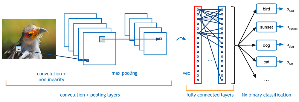 Diagram of a CNN layers. Source: https://adeshpande3.github.io/A-Beginner%27s-Guide-To-Understanding-Convolutional-Neural-Networks/
Layers in a ConvNet
There are four main operations in a standard ConvNet:
- Convolution
- Non Linearity (ReLU)
- Pooling or Sub Sampling
- Classification (Fully Connected Layer)
“This architecture is based on one of the very first convolutional neural networks, LeNet, which helped propel the field of Deep Learning. This pioneering work by Yann LeCun was named LeNet5 after many previous successful iterations since the year 1988″. [5] An Intuitive Explanation of Convolutional Neural Networks
Convolution Layer: An input image is a matrix of pixels, HxWxC, H for Height, W for Width and C for Channel. Grayscale images have only 1 channel while RGB or colored images have 3 channel: Red, Green and Blue. In a Conv layer only a small region in the input image is considered, computing a dot product with the weights and producing a single value. This operation called convolution preserves the spatial relationship between pixels in the image by learning image features on that small square of the input data.
The weights or CONV layer’s parameters consist of a set of learnable filters or kernels or features detector. The kernel is slidden across the whole image from the left-top corner to the right-bottom one, computing dot products between the weights of the filter and the pixels of the image covered by the kernel (called receptive field). Next step would be move the filter to the right by 1 unit, then right again by 1, when stride equals 1, and so on. For a 32x32x3 image and 12 kernels of 5x5x3 and a stride of 1, the output will be a 28x28x12 vector called a ‘feature map’ or ‘activation map’. For a HxWxC image, K kernels of HkxWkxC and stride s, the output would be H-Hk+s x W-Wk+s x K, we are considering zero padding.
 Note that the 3×3 matrix “sees” only a part of the input image in each stride.
A filter (with red outline) slides over the input image (convolution operation) to produce a feature map. The convolution of another filter (with the green outline), over the same image gives a different feature map as shown. It is important to note that the Convolution operation captures the local dependencies in the original image. Also notice how these two different filters generate different feature maps from the same original image.
But, what are the values of the filters? They are the parameters or weights and they are learnt by their own in the training phase.
- RELU Layer o Activation Layer: An additional operation called activation has been used after every convolution operation. ReLU stands for Rectified Linear Unit and is a non-linear operation. Its output is given by:

It will apply an element-wise activation function, such as the max(0,x) thresholding at zero, so replaces all negative pixel values in the feature map by zero. It provides non-linearity to our model that is mandatory because usually real-world data we want our ConvNet to learn would be non-linear. This operation do not change the size of the output.
 Applying a RELU function. Source [8]
Pooling Layer: “This layer is periodically included between Conv layers to reduce the amount of parameters, the spatial size of the model and the computational cost. This is why it is called subsampling or downsamplig. And most important it will help to prevent or control overfitting. The Pooling Layer operates independently on every depth slice of the input and resizes it spatially, usually using the MAX or AVG operation. it takes the largest element (MAX) or the average (AVG) from the rectified feature map within a defined window. The most common window form is a 2×2 pooling layer with a stride of 2. In our example, an input of 28x28x12 produce a 14x14x12 output”. Full explanation on this link [2] Convolutional Neural Networks for Visual Recognition: http://cs231n.github.io/convolutional-networks/
In the next image we can observed the application of a 2×2 pooling layer to a feature map.

“In addition to reduce the feature dimensions and the number of parameters, pooling layers makes the network invariant to small transformations, rotations, scaling, distortions and translations in the input image. This helps to detect objects in an image no matter where they are located”. Source [5] An Intuitive Explanation of Convolutional Neural Networks by ujjwalkarn.
Each filter composes a local patch of lower-level features into higher-level representation. That’s why CNNs are so powerful in Computer Vision.
Fully Connected Layer: “In a classification image problem, this layer basically takes an input whatever the output is of the conv or ReLU or pool layer preceding it and outputs an N dimensional vector where N is the number of classes that the program has to choose from. The output from the convolutional and pooling layers represent high-level features of the input image. The purpose of the Fully Connected layer is to use these features for classifying the input image into various classes based on the training dataset.”. See an extended explanation on [3] A Beginner’s Guide To Understanding Convolutional Neural Networks https://adeshpande3.github.io/A-Beginner%27s-Guide-To-Understanding-Convolutional-Neural-Networks/
A fully connected layer improves the predictive power of the Conv layers by learning non-linear combinations of the feature maps from the previous layers.
Intuition behind a CNN
In general, a way to understand how a CNN works is that every convolutional layer detects more complicated features than the layer before. In the first layer a ConvNet may learn to detect edges in diferent positions from raw pixels, then use the edges to detect simple shapes, as corners, in the second layer, and then use these shapes to deter higher-level features, such as facial shapes in higher layers [4].
 Learned features from a Convolutional Deep Belief Network. Source [9]
For example, we can detect edges by taking the values −1 and 1 on two adjacent pixels, and zero everywhere else. That is, we subtract two adjacent pixels. When side by side pixels are similar, this is gives us approximately zero. On edges, however, adjacent pixels are very different in the direction perpendicular to the edge. Then each layer applies different filters, typically hundreds or thousands like the ones showed above, and combines their results
A big argument for CNNs is that they are fast. Very fast. Convolutions are a central part of computer graphics and implemented on a hardware level on GPUs.
About the challenge
Our goal is to predict the accent of the speaker from spectrograms of speech samples. There are 3 accents to identity, people from Canada, India and England. We will use a CNN model to predict the accent of a given spectrograms.
We will continue in Part 2. describing and developing a CNN built with Keras framework and then it will be trained in Azure ML Services.
References:
[1] Description of the problem and the competition: https://datasciencecapstone.org/competitions/16/identifying-accents-speech/page/49/
[2] Convolutional Neural Networks for Visual Recognition: http://cs231n.github.io/convolutional-networks/
[3] A Beginner’s Guide To Understanding Convolutional Neural Networks https://adeshpande3.github.io/A-Beginner%27s-Guide-To-Understanding-Convolutional-Neural-Networks/
[4] Understanding Convolutional Neural Networks for NLP http://www.wildml.com/2015/11/understanding-convolutional-neural-networks-for-nlp/
[5] An Intuitive Explanation of Convolutional Neural Networks by ujjwalkarn, https://ujjwalkarn.me/2016/08/11/intuitive-explanation-convnets/
[6] Gradient-based Learning Applied to Document Recognition. Yann Lecun, León Bottou, Yoshua Bengio and Patrick Haffner. http://yann.lecun.com/exdb/publis/pdf/lecun-01a.pdf
[7] Deep Learning Methods for Vision CVPR 2012 Tutorial https://cs.nyu.edu/~fergus/tutorials/deep_learning_cvpr12/
[8] http://mlss.tuebingen.mpg.de/2015/slides/fergus/Fergus_1.pdf
[9] Convolutional Deep Belief Networks for Scalable Unsupervised Learning of Hierarchical Representations http://web.eecs.umich.edu/~honglak/icml09-ConvolutionalDeepBeliefNetworks.pdf
[10] Understanding Convolutions http://colah.github.io/posts/2014-07-Understanding-Convolutions/
[6] https://www.pyimagesearch.com/2018/11/26/instance-segmentation-with-opencv/